The recent rise of diffusion-based models

Introduction

Every fan of generative modeling has been living an absolute dream for the last year and a half (at least!). The past few months have brought several developments and papers on text-to-image generation, each one arguably better than the last. We have observed a social media surge of spectacular, purely AI-generated images, such as this golden retriever answering tough questions on the campaign trail or a brain riding a rocketship to the moon.

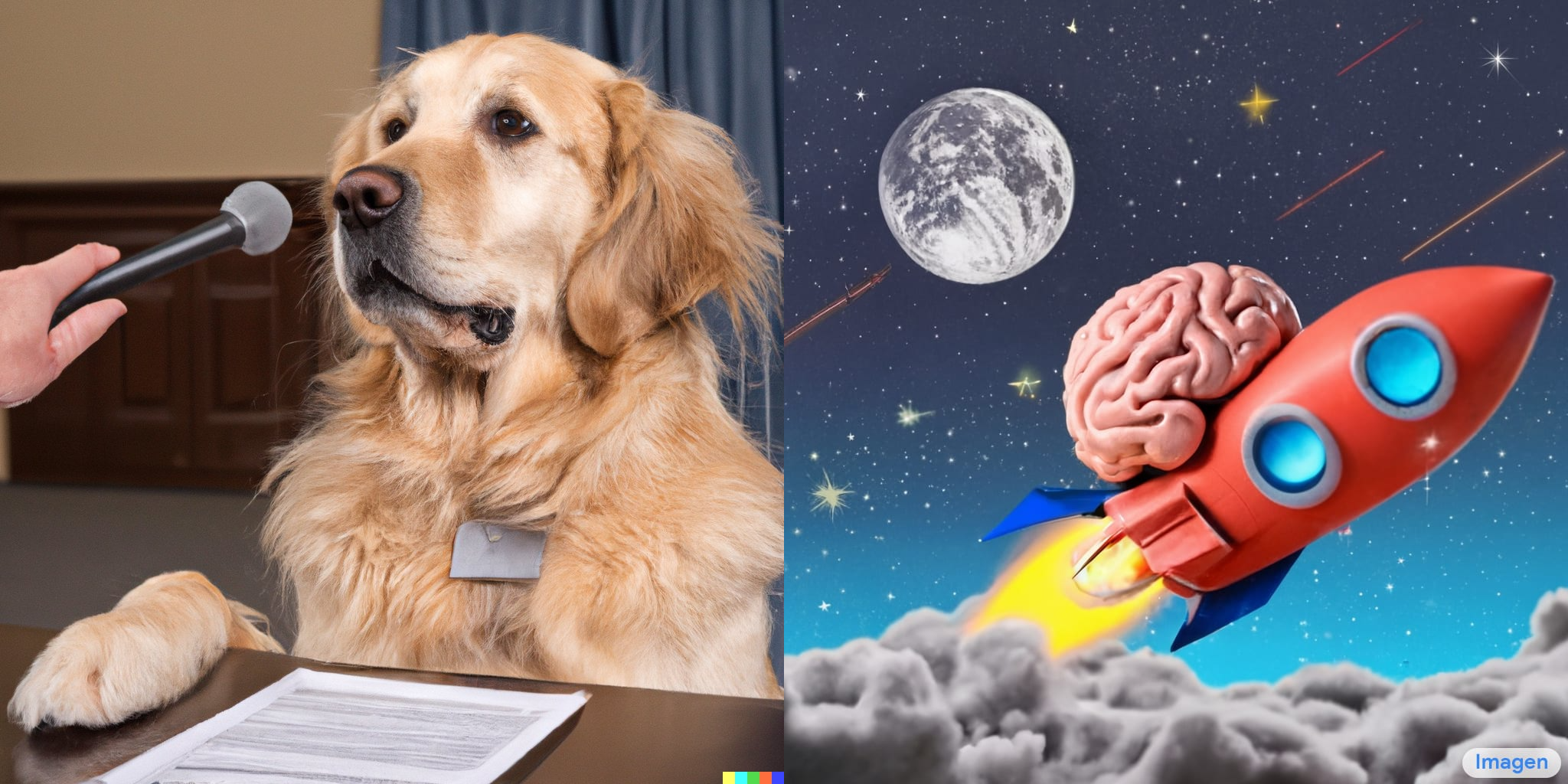
Sources: https://openai.com/dall-e-2/ and https://imagen.research.google/

In this post, we will sum up the very recent history of solving the text-to-image generation problem and explain the latest developments regarding diffusion models, which are playing a huge role in the new, state-of-the-art architectures.

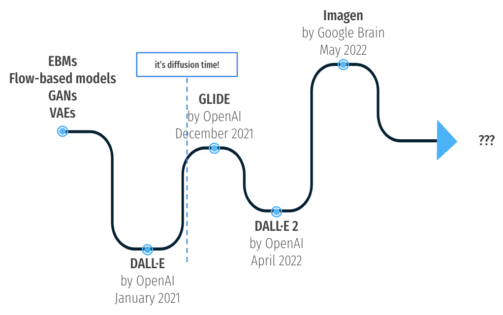
Short timeline of image generation and text-to-image solutions. Source: author

It all starts with DALL·E

In 2020 the OpenAl team [1] published the GPT-3 model - a multimodal do-it-all huge language model, capable of machine translation, text generation, semantic analysis etc. The model swiftly became regarded as the state-of-the-art for language modeling solutions, and DALL·E [7] can be viewed as a natural expansion of the transformer capabilities into the computer vision domain. Below is a brief reminder of how DALL·E works.

Autoregressive approach

The authors proposed an elegant two-stage approach:

train a discrete VAE model to compress images into image tokens,
concatenate the encoded text snippet with the image tokens and train the autoregressive transformer to learn the joint distribution over text and images.

The final version was trained on 250 million text-image pairs obtained from the Internet.

CLIP

During inference, the model is able to output a whole batch of generated images. But how can we estimate which images are best? Simultaneously with the publication of DALL·E, the OpenAI team presented a solution for image and text linking called CLIP [9]. In a nutshell, CLIP offers a reliable way of pairing a text snippet with its image representation. Putting aside all of the technical aspects, the idea of training this type of model is fairly simple - take the text snippet and encode it, take an image and encode it. Do that for a lot of examples (400 million (image, text) pairs) and train the model in a contrastive fashion.

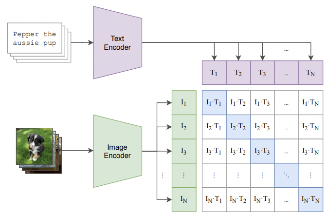
Visualisation of CLIP contrastive pre-training, source: [9]

This kind of mapping allows us to estimate which of the generated images are the best match considering the text input. DALL·E attracted major attention from people both inside and outside the AI world; it gained lots of publicity and stirred a great deal of conversation. Even so, it only gets an honorable mention here, as the trends shifted quite quickly towards novel ideas.

All you need is diffusion

Sohl-Dickstein et al. [2] proposed a fresh idea on the subject of image generation - diffusion models.

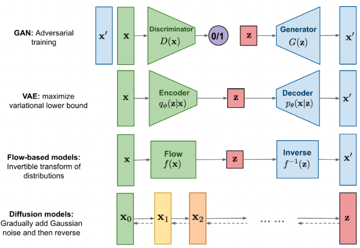
Generative models, source: [13]

The idea is inspired by non-equilibrium thermodynamics, although underneath it is packed with some interesting mathematical concepts. We can notice the already known concept of encoder-decoder structure here, but the underlying idea is a bit different than what we can observe in traditional variational autoencoders. To understand the basics of this model, we need to describe forward and reverse diffusion processes.

Forward image diffusion

This process can be described as gradually applying Gaussian noise to the image until it becomes entirely unrecognizable. This process is fixed in a stochastic sense - the noise application procedure can be formulated as the Markov chain of sequential diffusion steps. To untangle the difficult wording a little bit, we can neatly describe it with a few formulas. Assume that images have a certain starting distribution $q(\bf{x}_{0})$. We can sample just one image from this distribution - $\bf{x}_{0}$. We want to perform a chain of diffusion steps $\bf{x}_{0} \to \bf{x}_{1} \to ... \to \bf{x}_{\it{T}}$ , each step disintegrating the image more and more.

How exactly is the noise applied? It is formally defined by a noising schedule $\{\beta_{t}\}^{T}_{t=1}$, where for every $t = 1,...,T$ we have $\beta_{t} \in (0,1)$. With such a schedule we can formally define the forward process as

\[q\left(\mathbf{x}_{t} \mid \mathbf{x}_{t-1}\right)=\mathcal{N}\left(\sqrt{1-\beta_{t}} \mathbf{x}_{t-1}, \beta_{t} \mathbf{I}\right).\]

There are just two more things worth mentioning:

As the number of noising steps is going up $(T \to \infty)$, the final distribution $q(\mathbf{x}_{T})$ approaches a very handy isotropic Gaussian distribution. That makes any future sampling from noised distribution efficient and easy.
Noising with Gaussian kernel provides another benefit - there is no need to walk step-by-step through noising process to achieve any intermediate latent state. We can sample them directly thanks to reparametrization
\[q\left(\mathbf{x}_{t} \mid \mathbf{x}_{0}\right)=\mathcal{N}\left(\sqrt{\bar{\alpha}_{t}} \mathbf{x}_{0},\left(1-\bar{\alpha}_{t}\right) \mathbf{I}\right) = \sqrt{\bar{\alpha}_{t}} \mathbf{x}_{0}+\sqrt{1-\bar{\alpha}_{t}} \cdot \epsilon,\]
where $\alpha_{t} := 1-\beta_{t}$, $\bar{\alpha}_{t} := \prod_{k=0}^{t}\alpha_{k}$ and $\epsilon \sim \mathcal{N}(0, \mathbf{I})$. Here $\epsilon$ represents Gaussian noise - this formulation will be essential for the model training.

Reverse image diffusion

We have a nicely defined forward process. One might ask - so what? Why can’t we just define a reverse process $q\left(\mathbf{x}_{t-1} \mid \mathbf{x}_{t}\right)$ and trace back from the noise to the image? First of all, that would fail conceptually, as we want to have a neural network that learns how to deal with a problem - we shouldn’t provide it with a clear solution. And second of all, we cannot quite do that, as it would require marginalization over the entire data distribution. To get back to the starting distribution $q(\bf{x}_{0})$ from the noised sample we would have to marginalize over all of the ways we could arise at $\mathbf{x}_{0}$ from the noise, including all of the latent states. That means calculating $\int q(\mathbf{x}_{0:T})d\mathbf{x}_{1:T}$, which is intractable. So, if we cannot calculate it, surely we can… approximate it!

The core idea is to develop a reliable solution - in the form of a learnable network - that successfully approximates the reverse diffusion process. The first way to achieve that is by estimating the mean and covariance for denoising steps

\[p_{\theta}\left(\mathbf{x}_{t-1} \mid \mathbf{x}_{t}\right)=\mathcal{N}(\mu_{\theta}(\mathbf{x}_{t}, t), \Sigma_{\theta}(\mathbf{x}_{t}, t) ).\]

In a practical sense, $\mu_{\theta}(\mathbf{x}_{t}, t)$ can be estimated via neural network and $\Sigma_{\theta}(\mathbf{x}_{t}, t)$ can be fixed to a certain constant related with the noising schedule, such as $\beta_{t}\mathbf{I}$.

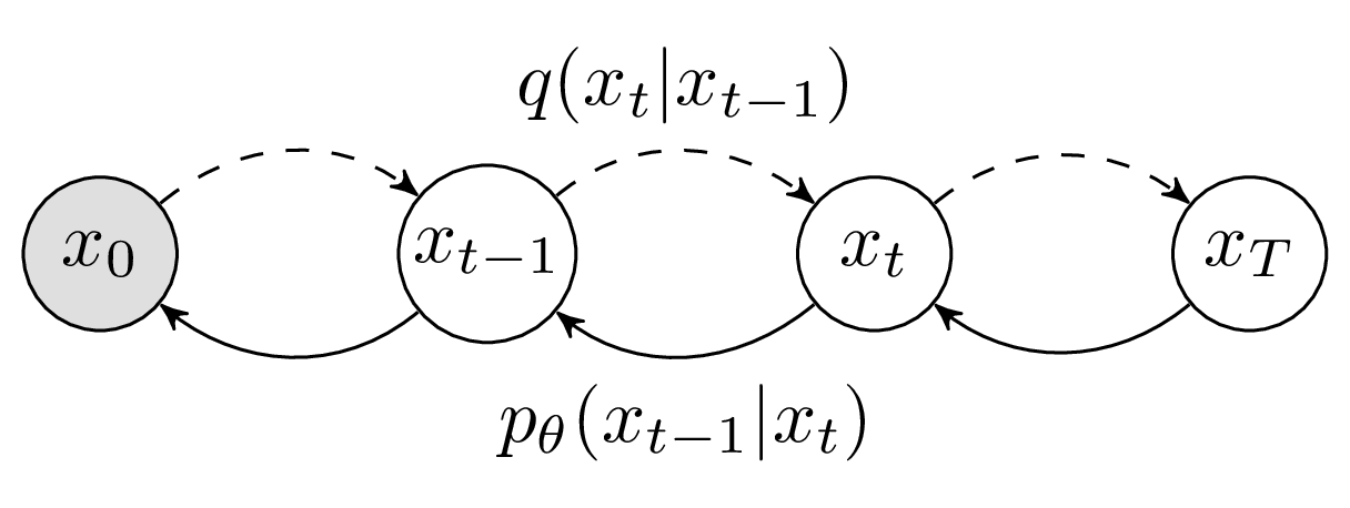
Forward and reverse diffusion processes, source: [14]

Estimating $\mu_{\theta}(\mathbf{x}_{t}, t)$ this way is possible, but Ho et al. [3] came up with a different way of training - a neural network $\epsilon_{\theta}(\mathbf{x}_{t}, t)$ can be trained to predict the noise $\epsilon$ from the earlier formulation of $q\left(\mathbf{x}_{t} \mid \mathbf{x}_{0}\right)$.

As in Ho et al. [3], the training process consists of steps:

Sample image $\mathbf{x}_{0}\sim q(\bf{x}_{0})$,
Choose a certain step in diffusion process $t \sim U(\{1,2,...,T\})$,
Apply the noising $\epsilon \sim \mathcal{N}(0,\mathbf{I})$,
Try to estimate the noise $\epsilon_{\theta}(\mathbf{x}_{t}, t)= \epsilon_{\theta}(\sqrt{\bar{\alpha}_{t}} \mathbf{x}_{0}+\sqrt{1-\bar{\alpha}_{t}} \cdot \epsilon, t)$,
Learn the network by gradient descent on loss $\nabla_{\theta} \|\epsilon - \epsilon_{\theta}(\mathbf{x}_{t}, t)\|^{2}$.

In general, loss can be nicely presented as

\[L_{\text{diffusion}}=\mathbb{E}_{t, \mathbf{x}_{0}, \epsilon}\left[\left\|\epsilon-\epsilon_{\theta}\left(\mathbf{x}_{t}, t\right)\right\|^{2}\right],\]

where $t, \mathbf{x}_0$ and $\epsilon$ are described as in the steps above.

All of the formulations, reparametrizations and derivations are a bit math-extensive, but there are already some great resources available for anyone that wants to have a deeper understanding of the subject. Most notably, Lillian Weng [13], Angus Turner [14] and Ayan Das [15] went through some deep derivations while maintaining an understandable tone - I highly recommend checking these posts.

Guiding the diffusion

The above part itself explains how we can perceive the diffusion model as generative. Once the model $\epsilon_{\theta}(\mathbf{x}_{t}, t)$ is trained, we can use it to run the noise $\mathbf{x}_{t}$ back to $\mathbf{x}_{0}$. Given that it is straightforward to sample the noise from isotropic Gaussian distribution, we can obtain limitless image variations. We can also guide the image generation by feeding additional information to the network during the training process. Assuming that the images are labeled, the information about class $y$ can be fed into a class-conditional diffusion model $\epsilon_{\theta}(\mathbf{x}_{t}, t \mid y)$.

One way of introducing the guidance in the training process is to train a separate model, which acts as a classifier of noisy images. At each step of denoising, the classifier checks whether the image is denoised in the right direction and contributes its own gradient of loss function into the overall loss of diffusion model.

Ho & Salimans [5] proposed an idea on how to feed the class information into the model without the need to train an additional classifier. During the training the model $\epsilon_{\theta}(\mathbf{x}_{t}, t \mid y)$ is sometimes (with fixed probability) not shown the actual class $y$. Instead, the class label is replaced with the null label $\emptyset$. So it learns to perform diffusion with and without the guidance. For inference, the model performs two predictions, once given the class label $\epsilon_{\theta}(\mathbf{x}_{t}, t \mid y)$ and once not $\epsilon_{\theta}(\mathbf{x}_{t}, t \mid \emptyset)$. The final prediction of the model is moved away from $\epsilon_{\theta}(\mathbf{x}_{t}, t \mid \emptyset)$ and towards $\epsilon_{\theta}(\mathbf{x}_{t}, t \mid y)$ by scaling with guidance scale $s \geqslant 1$.

\[\hat{\epsilon}_{\theta}\left(\mathbf{x}_{t}, t \mid y\right)=\epsilon_{\theta}\left(\mathbf{x}_{t}, t \mid \emptyset\right)+s \cdot\left(\epsilon_{\theta}\left(\mathbf{x}_{t}, t \mid y\right)-\epsilon_{\theta}\left(\mathbf{x}_{t}, t \mid \emptyset\right)\right)\]

This kind of classifier-free guidance uses only the main model’s comprehension - an additional classifier is not needed - which yields better results according to Nichol et al. [6].

Text-guided diffusion with GLIDE

Even though the paper describing GLIDE [6] architecture received the least publicity out of all the publications discussed in this post, it arguably presents the most novel and interesting ideas. It combines all of the concepts presented in the previous chapter nicely. We already know how diffusion models work and that we can use them to generate images. The two questions we would now like to answer are:

How can we use the textual information to guide the diffusion model?
How can we make sure that the quality of the model is good enough?

Architecture choice

Architecture can be boiled down to three main components:

A UNet based model responsible for the visual part of the diffusion learning,
A transformer-based model responsible for creating a text embedding from a snippet of text,
An upsampling diffusion model is used for enhancing output image resolution.

The first two work together in order to create a text-guided image output, while the last one is used to enlarge the image while preserving the quality.

The core of the model is the well-known UNet architecture, used for the diffusion in Dhariwal & Nichol [8]. The model, just like in its early versions, stacks residual layers with downsampling and upsampling convolutions. It also consists of attention layers which are crucial for simultaneous text processing. The model proposed by the authors has around 2.3 billion parameters and was trained on the same dataset as DALL·E.

The text used for guidance is encoded in tokens and fed into the Transformer model. The model used in GLIDE had roughly 1.2 billion parameters and was built from 24 residual blocks of width 2048. The output of the transformer has two purposes:

the final embedding token is used as class embedding $y$ in $\epsilon_{\theta}(\mathbf{x}_{t}, t \mid y)$,
the final layer of token embeddings is added to every attention layer of the model.

It is clear that a great deal of focus was put into making sure that the model receives enough text-related context in order to generate accurate images. The model is conditioned on the text snippet embedding, the encoded text is concatenated with the attention context and during training, the classifier-free guidance is used.

As for the final component, the authors used the diffusion model to go from a low-resolution to a high-resolution image using an ImageNet upsampler.

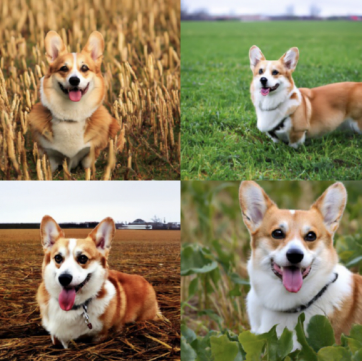
GLIDE interpretation of ‘a corgi in a field’, source: [6]

GLIDE incorporates a few notable achievements developed in recent years and sheds new light on the concept of text-guided image generation. Given that the DALL·E model was based on different structures, it is fair to say that the publication of GLIDE represents the dawn of the diffusion-based text-to-image generation era.

DALL·E 2

The OpenAI team doesn’t seem to get much rest, as in April they took the Internet by storm with DALL·E 2 [7]. It takes elements from both predecessors: it relies heavily on CLIP [9] but a large part of the solution revolves around GLIDE [6] architecture. DALL·E 2 has two main underlying components called the prior and the decoder, which are able to produce image output when stacked together. The entire mechanism was named unCLIP, which may already spoil the mystery of what exactly is going on under the hood.

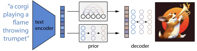
Visualization of DALL·E 2 two-stage mechanism. Source: [7]

The prior

The first stage is meant to convert the caption - a text snippet such as a “corgi playing a flame-throwing trumpet” - into text embedding. We obtain it using a frozen CLIP model.

After text embedding comes the fun part - we now want to obtain an image embedding, similar to the one which is obtained via the CLIP model. We want it to encapsulate all important information from the text embedding, as it will be used for image generation through diffusion. Well, isn’t that exactly what CLIP is for? If we want to find a respective image embedding for our input phrase, we can just look at what is close to our text embedding in the CLIP encoded space. One of the authors of DALL·E 2 posted a nice explanation of why that solution fails and why the prior is needed - “An infinite number of images could be consistent with a given caption, so the outputs of the two encoders will not perfectly coincide. Hence, a separate prior model is needed to “translate” the text embedding into an image embedding that could plausibly match it”.

On top of that, the authors empirically checked the importance of the prior in the network. Passing both the image embedding produced by the prior and the text vastly outperforms generation using only the caption or caption with CLIP text embedding.

Samples generated conditioned on: caption, text embedding and image embedding. Source: [7]

The authors tested two model classes for the prior: the autoregressive model and the diffusion model. This post will cover only the diffusion prior, as it was deemed better performing than autoregressive, especially from a computational point of view. For the training of prior, a decoder-only Transformer model was chosen. It was trained by using a sequence of several inputs:

encoded text,
CLIP text embedding,
embedding for the diffusion timestep,
noised image embedding,

with the goal of outputting an unnoised image embedding $z_{i}$. As opposed to the way of training proposed by Ho et al.[7] covered in previous sections, predicting the unnoised image embedding directly instead of predicting the noise was a better fit. So, remembering the previous formula for diffusion loss in a guided model

\[L_{\text{diffusion}}=\mathbb{E}_{t, \mathbf{x}_{0}, \epsilon}\left[\left\|\epsilon-\epsilon_{\theta}\left(\mathbf{x}_{t}, t\mid y\right)\right\|^{2}\right],\]

we can present the prior diffusion loss as

\[L_{\text{prior:diffusion}}=\mathbb{E}_{t}\left[\left\|z_{i}-f_{\theta}\left({z}_{i}^{t}, t \mid y\right)\right\|^{2}\right],\]

where $f_{\theta}$ stands for the prior model, ${z}_{i}^{t}$ is the noised image embedding, $t$ is the timestamp and $y$ is the caption used for guidance.

The decoder

We covered the prior part of the unCLIP, which was meant to produce a model that is able to encapsulate all of the important information from the text into a CLIP-like image embedding. Now we want to use that image embedding to generate an actual visual output. This is when the name unCLIP unfolds itself - we are walking back from the image embedding to the image, the reverse of what happens when the CLIP image encoder is trained.

As the saying goes: “After one diffusion model it is time for another diffusion model!”. And this one we already know - it is GLIDE, although slightly modified. Only slightly, since the single major change is adding the additional CLIP image embedding (produced by the prior) to the vanilla GLIDE text encoder. After all, this is exactly what the prior was trained for - to provide information for the decoder. Guidance is used just as in regular GLIDE. To improve it, CLIP embeddings are set to $\emptyset$ in 10% of cases and text captions $y$ in 50% of cases.

Another thing that did not change is the idea of upsampling after the image generation. The output is tossed into additional diffusion-based models. This time two upsampling models are used (instead of one in the original GLIDE), one taking the image from 64x64 to 256x256 and the other further enhancing resolution up to 1024x1024.

Imagen

The Google Brain team decided not to be late to the party, as less than two months after the publication of DALL·E 2 they presented the fruits of their own labor - Imagen (Saharia et al. [7]).

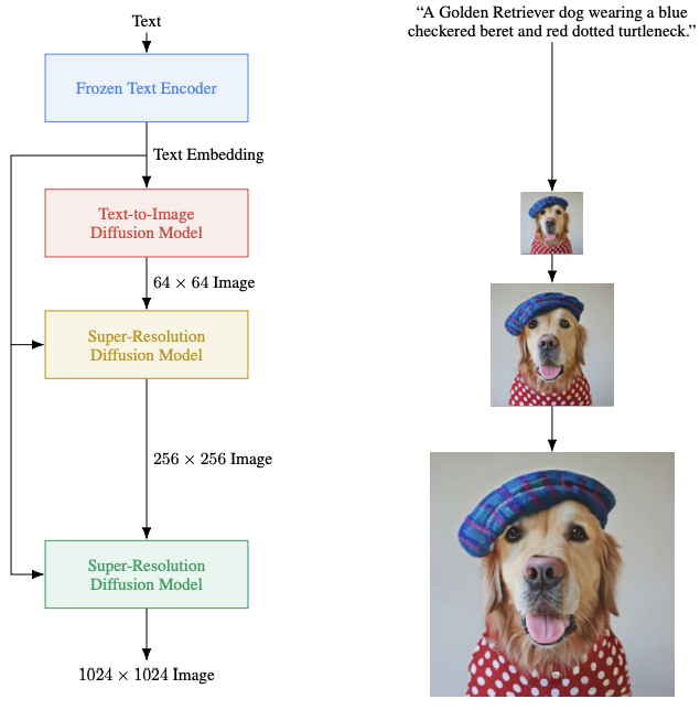
Overview of Imagen architecture. Source: [7]

Imagen architecture seems to be oddly simple in its structure. A pretrained textual model is used to create the embeddings that are diffused into an image. Next, the resolution is increased via super-resolution diffusion models - the steps we already know from DALL·E 2. A lot of novelties are scattered in different bits of the architecture - a few in the model itself and several in the training process. Together, they offer a slight upgrade when compared to other solutions. Given the large portion of knowledge already served, we can explain this model via differences with previously described models:

Use a pretrained transformer instead of training it from scratch.

This is viewed as the core improvement compared to OpenAI’s work. For everything regarding text embeddings, the GLIDE authors used a new, specifically trained transformer model. The Imagen authors used a pretrained, frozen T5-XXL model [4]. The idea is that this model has vastly more context regarding language processing than a model trained only on the image captions, and so is able to produce more valuable embeddings without the need to additionally fine-tune it.

Make the underlying neural network more efficient.

An upgraded version of the neural network called Efficient U-net was used as the backbone of super-resolution diffusion models. It is said to be more memory-efficient and simpler than the previous version, and it converges faster as well. The changes were introduced mainly in residual blocks and via additional scaling of the values inside the network. For anyone who enjoys digging deep into the details - the changes are well documented in Saharia et al. [7].

Use conditioning augmentation to enhance image fidelity.

Since the solution can be viewed as a sequence of diffusion models, there is an argument to be made about enhancements in the areas where the models are linked. Ho et al. [10] presented a solution called conditioning augmentation. In simple terms, it is equivalent to applying various data augmentation techniques, such as a Gaussian blur, to a low-resolution image before it is fed into the super-resolution models.

There are a few other resources deemed crucial to a low FID score and high image fidelity (such as dynamic thresholding) - these are explained in detail in the source paper [7]. The core of the approach is already covered in previous chapters.

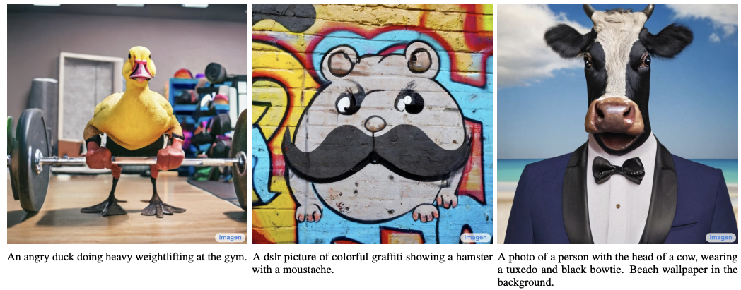
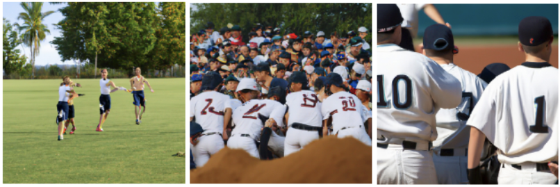
Some of Imagen generations with captions. Source: [7]

Is it the best yet?

As of writing this text, Google’s Imagen is considered to be state-of-the-art as far as text-to-image generation is concerned. But why exactly is that? How can we evaluate the models and compare them to each other?

The authors of Imagen opted for two means of evaluation. One is considered to be the current standard for text-to-image modeling, namely establishing a Fréchet inception distance score on a COCO validation dataset. The authors report (unsurprisingly) that Imagen shows a state-of-the-art performance, its zero-shot FID outperforming all other models, even those specifically trained on COCO.

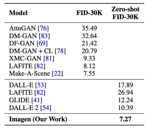
Comparison of several models. Source: [7]

A far more intriguing means of evaluation is a brand new proposal from the authors called DrawBench - a comprehensive and challenging set of prompts that support the evaluation and comparison of text-to-image models (source). It consists of 200 prompts divided into 11 categories, collected from e.g. DALL·E or Reddit. A list of the prompts with categories can be found in [17]. The evaluation was performed by 275 unbiased (sic!) raters, 25 for each category. Each rater was shown two non-cherry picked and random sets of images generated by two different models (e.g. Imagen and DALL·E 2) and had to respond to two questions:

Which set of images is of higher quality?
Which set of images better represents the text caption?

These two questions are meant to address the two most important characteristics of a good text-to-image model: the quality of the images produced (fidelity) and how well it reflects the input text prompt (alignment). Each rater had three choices - to claim that one of the models performs better, or to call it a tie. Once again, there can be only one winner. Interestingly, the GLIDE model seems to perform slightly better than DALL·E 2, at least based on this curated dataset.

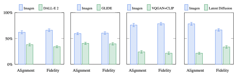
Imagen vs other models. Source: [7]

As expected, a large portion of the publication is devoted to the comparison between the images produced by Imagen and GLIDE/DALL·E - more can be found in Appendix E of [7].

The fun is far from over

As usual, with new architecture gaining recognition there is a surge of interesting publications and solutions emerging from the void. The pace of developments makes it nearly impossible to track every interesting publication. There are also a lot of interesting characteristics of the models to discover other than raw generative power, such as image inpainting, style transfer, and image editing.

Apart from the understandable excitement over a new era of generative models, there are some shortcomings embedded into the diffusion process structure, such as slow sampling speed compared to previous models [16].

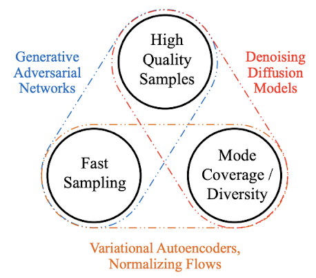
Models comparison. Source: [16]

For anyone who likes to go deep into the minutiae of implementation, I highly recommend going through Phil Wang’s (@lucidrains on github) repositories [20], which is a collaborative effort from many people to recreate the unpublished models in PyTorch.

For anyone who would like to admire some more examples of DALL·E 2’s generative power, I recommend checking the newly created subreddit with DALL·E 2 creations in [18]. It is moderated by people with OpenAI’s Lab access - feel free to join the waitlist [19] and have the opportunity to play with models yourself.